Logistic regression is the best regression approach to utilize when the dependent variable is dichotomous (binary). Like other regression studies, logistic regression is a predictive analysis. Logistic regression is a statistical approach for defining and explaining the relationship between one dependent binary variable and one or more independent variables that are nominal, ordinal, interval, or ratio-level.

The Iris flower data set is a multivariate data set created in 1936 by British statistician and biologist Ronald Fisher in his paper The use of multiple measures in taxonomic concerns. Because Edgar Anderson gathered the information to quantify the morphologic variation of three related species of Iris blooms, it is commonly known to as Anderson’s Iris data set. Each of the three Iris species is represented by 50 samples in the data set (Iris Setosa, Iris virginica, and Iris versicolor). The length and width of the sepals and petals in centimeters were measured for each sample.
This dataset serves as a common test case for a variety of machine learning statistical classification techniques.
Download Dataset: https://www.kaggle.com/datasets/arshid/iris-flower-dataset?select=IRIS.csv
Program Used:


or you can use Jupyter Notebook
Procedures
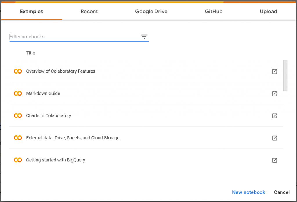
1. Open Google Collaboratory
2. Click open “New notebook”
3. After making new notebook. The code is provided as reference below:
STEPS OF CODING:
a. Import the important packages
For this exercise it require the Pandas package for loading the data, the matplotlib package for plotting as well as scitkit-learn for creating the Logistic Regression model. Import all of the required packages and relevant modules for these tasks.
import pandas as pd
import matplotlib.pyplot as plt
from sklearn.linear_model import LogisticRegression
b. Load the data
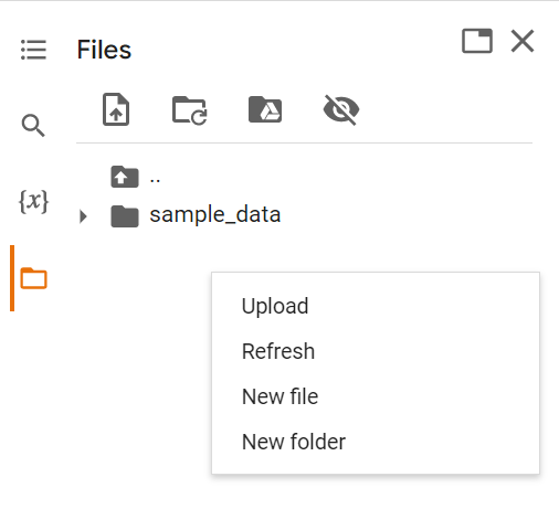
Note: Upload your dataset first in the file section. Make sure the file name of your dataset are same in the code.
data = pd.read_csv('IRIS.csv')
data.head()
c. Feature Engineering
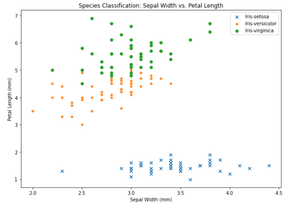
We must choose the characteristics that will produce the most powerful categorization model. Plot a variety of characteristics against the assigned species categories, for example. Sepal Length vs. Petal Length and Species. Examine the charts visually for any patterns that might suggest separation of the species.
markers = {
    'Iris-setosa' : {'marker' : 'x'},
    'Iris-versicolor' : {'marker' : '*'},
    'Iris-virginica' : {'marker' : 'o'},
}
plt.figure(figsize=(10, 7))

for name, group in data.groupby('species'):
    plt. scatter(group['sepal_width'], group['petal_length'],
                 label = name, marker = markers[name]['marker'],)

    plt.title('Species Classification: Sepal Width vs. Petal Length')
    plt.xlabel('Sepal Width (mm)'); plt.ylabel('Petal Length (mm)')
    plt.legend();
Output:
Select the features by writing the column names in the list below:
selected_features = ['sepal_width', 'petal_length'] d. Constructing Logistic Regression
Before we can construct the model we must first convert the species values into labels that can be used within the model. Replace:
- The species string Iris-setosa with the value 0
- The species string Iris-versicolor with the value 1
- The species string Iris-virginica with the value 2
species = [ 'Iris-setosa', 'Iris-versicolor', 'Iris-virginica']
output = [species. index(spec) for spec in data.species]
Create the model using the selected_features and the assigned species labels
model=LogisticRegression(multi_class='auto', solver='lbfgs')
model.fit(data [selected_features], output)
Compute the accuracy of the model against the training set:
model.score(data[selected_features], output) Output: 0.9533333333333334
Construct another model using your second choice selected_features and compare the performance:
selected_features = ['sepal_length', 'petal_width']
model.fit(data [selected_features], output)
model.score(data [selected_features], output)
Output: 0.96
Construct another model using all available information and compare the performance:
selected_features = ['sepal_width', 'sepal_length', 'petal_width', 'petal_length']
model.fit(data [selected_features], output)
model.score(data [selected_features], output)
Output: 0.9733333333333334
selected_features = ['petal_width', 'petal_length']
model.fit(data [selected_features], output)
model.score(data [selected_features], output)
Output: 0.9666666666666667
References:
https://www.statisticssolutions.com/free-resources/directory-of-statistical-analyses/what-is-logistic-regression/
https://www.kaggle.com/datasets/arshid/iris-flower-dataset